Examining Win Probabilities Playing Maexchen

Brief Game Rules

In this game you roll two dices. The higher dice represents the first digit, the lower one the second digit of your result. For example: 1,3 will get you 31; 2,5 will get you 52; 1,1 will get you 11.

The best Result one might get is 21 also called Mäxchen. The next highest results are the rolls, where both digits match (11,22,33,etc.) with 66 being the highest and therefore 11 the worst one. After that, the higher your roll the better.

Simulation

First we need to simulate the dice rolls. I usually write a function for one simulation, so I will do it here as well:

roll_game <- function() {
  r1 <- sample(6, 1)
  r2 <- sample(6, 1)

  if (r1 > r2) {
    r1 * 10 + r2
  } else {
    r2 * 10 + r1
  }
}

roll_game()

## [1] 32

roll_game()

## [1] 32

roll_game()

## [1] 61

I use the sample-Function to generate the dice rolls. After we generated each dice we need to order it to match the rules of the game. These two steps are all we need to do in order to simulate one roll of the game. Lets expand this to simulate a bunch of games.

simulation <- tibble(sim = 1:1e6) %>%
  mutate(roll = replicate(n(), roll_game()))

simulation

## # A tibble: 1,000,000 x 2
##      sim  roll
##    <int> <dbl>
##  1     1    22
##  2     2    32
##  3     3    54
##  4     4    53
##  5     5    54
##  6     6    65
##  7     7    63
##  8     8    31
##  9     9    64
## 10    10    62
## # ... with 999,990 more rows

Now we have generated a million rolls (in a few seconds).

order <- c(15, 21, 16, 1, 2, 17, 3, 4, 5, 18, 6, 7, 8, 9, 19, 10, 11, 12, 13, 14, 20)

dist <- simulation %>%
  count(roll) %>%
  mutate(
    prob = n / 1e6,
    roll = as.factor(roll),
    order = order
  ) %>%
  arrange(order)

dist

## # A tibble: 21 x 4
##    roll      n   prob order
##    <fct> <int>  <dbl> <dbl>
##  1 31    56058 0.0561     1
##  2 32    55932 0.0559     2
##  3 41    55889 0.0559     3
##  4 42    55449 0.0554     4
##  5 43    55083 0.0551     5
##  6 51    55332 0.0553     6
##  7 52    55687 0.0557     7
##  8 53    55580 0.0556     8
##  9 54    55673 0.0557     9
## 10 61    55367 0.0554    10
## # ... with 11 more rows

As explained before the game has a special order in which they results are sorted. The Vector order maps that sequence to the default numerical order, e.g. 31 is the 4th lowest number you can roll but is the worst result you can get in this game (11,21,22 are valued higher). We count the occurence of each dice result.

dist %>%
  mutate(roll = fct_inorder(roll)) %>%
  ggplot(aes(roll, prob)) +
  geom_col(fill = "darkred") +
  labs(
    title = "Probability Distribution for 'Mäxchen'",
    x = "Result",
    y = "Probability"
  ) +
  scale_y_continuous(labels = scales::percent_format()) +
  theme(axis.text.x = element_text(angle = 45, hjust = 1))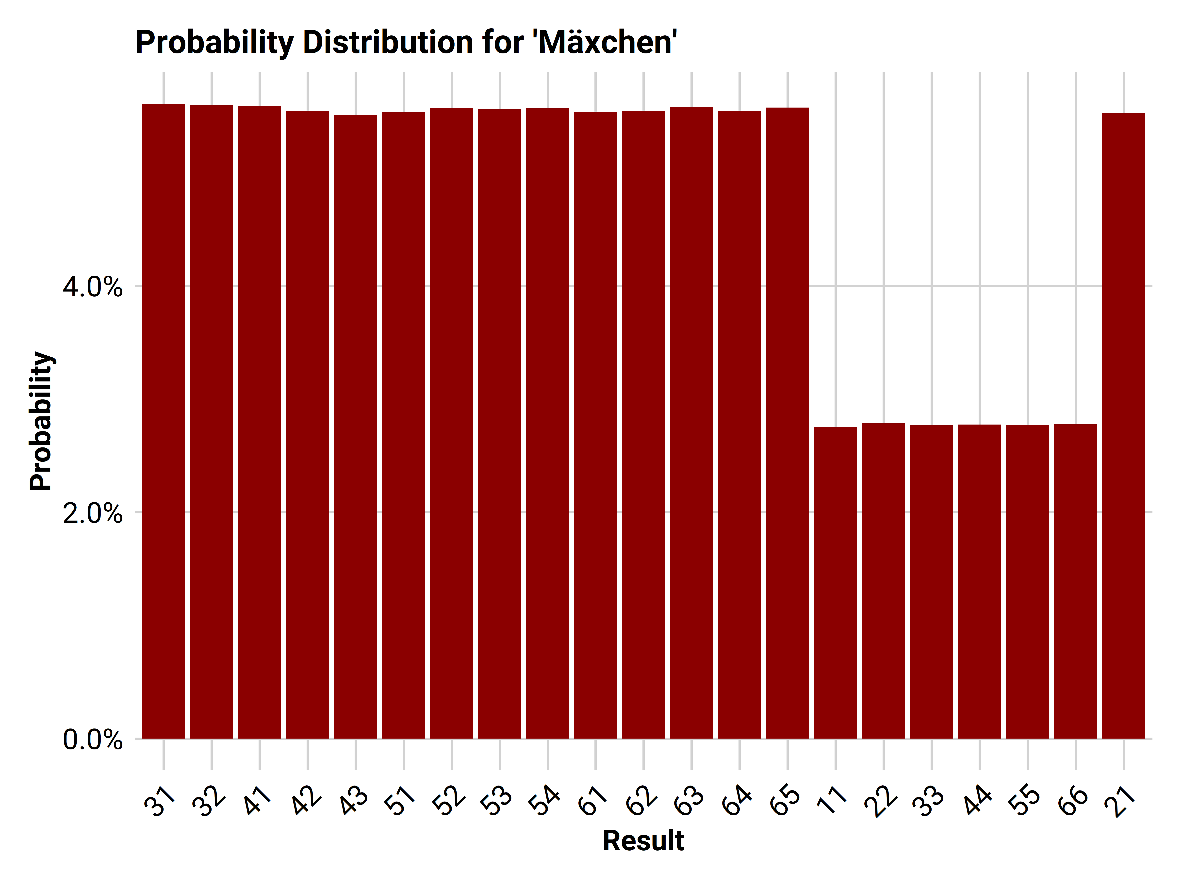

If you think about it, this result was pretty obvious. For every result without equal digits you have two ways of archiving it: first digit on first dice and second digit on second dice or the other way around. If your result has equal digits you only have one. Thus, the exact chance of every result is 5.556% or 2.778% for same digits results.

beat_prob <- dist %>%
  mutate(
    prob = ifelse(roll %in% c(11, 22, 33, 44, 55, 66), 1 / 36, 2 / 36),
    prob_sum = cumsum(prob),
    beat = 1 - prob_sum
  )
beat_prob

## # A tibble: 21 x 6
##    roll      n   prob order prob_sum  beat
##    <fct> <int>  <dbl> <dbl>    <dbl> <dbl>
##  1 31    56058 0.0556     1   0.0556 0.944
##  2 32    55932 0.0556     2   0.111  0.889
##  3 41    55889 0.0556     3   0.167  0.833
##  4 42    55449 0.0556     4   0.222  0.778
##  5 43    55083 0.0556     5   0.278  0.722
##  6 51    55332 0.0556     6   0.333  0.667
##  7 52    55687 0.0556     7   0.389  0.611
##  8 53    55580 0.0556     8   0.444  0.556
##  9 54    55673 0.0556     9   0.5    0.5  
## 10 61    55367 0.0556    10   0.556  0.444
## # ... with 11 more rows

Since we now know the exact probability we change our values from the simulation accordingly. We calculate the cumulative sum for every roll. This value represents how likely we roll something worse or as bad as the respective roll. Since we wanna know the probability to beat a roll we have to subtract the calculated probability from 1. Let’s plot the result:

beat_prob %>%
  mutate(roll = fct_inorder(roll)) %>%
  ggplot(aes(roll, beat)) +
  geom_col(fill = "darkred") +
  geom_text(aes(label = percent(beat)), family = "Roboto", vjust = -.8, size = 3) +
  labs(
    title = "Probability of beating a result in 'Mäxchen'",
    x = "Result",
    y = "Probability"
  ) +
  scale_y_continuous(labels = scales::percent_format()) +
  theme(axis.text.x = element_text(angle = 45, hjust = 1))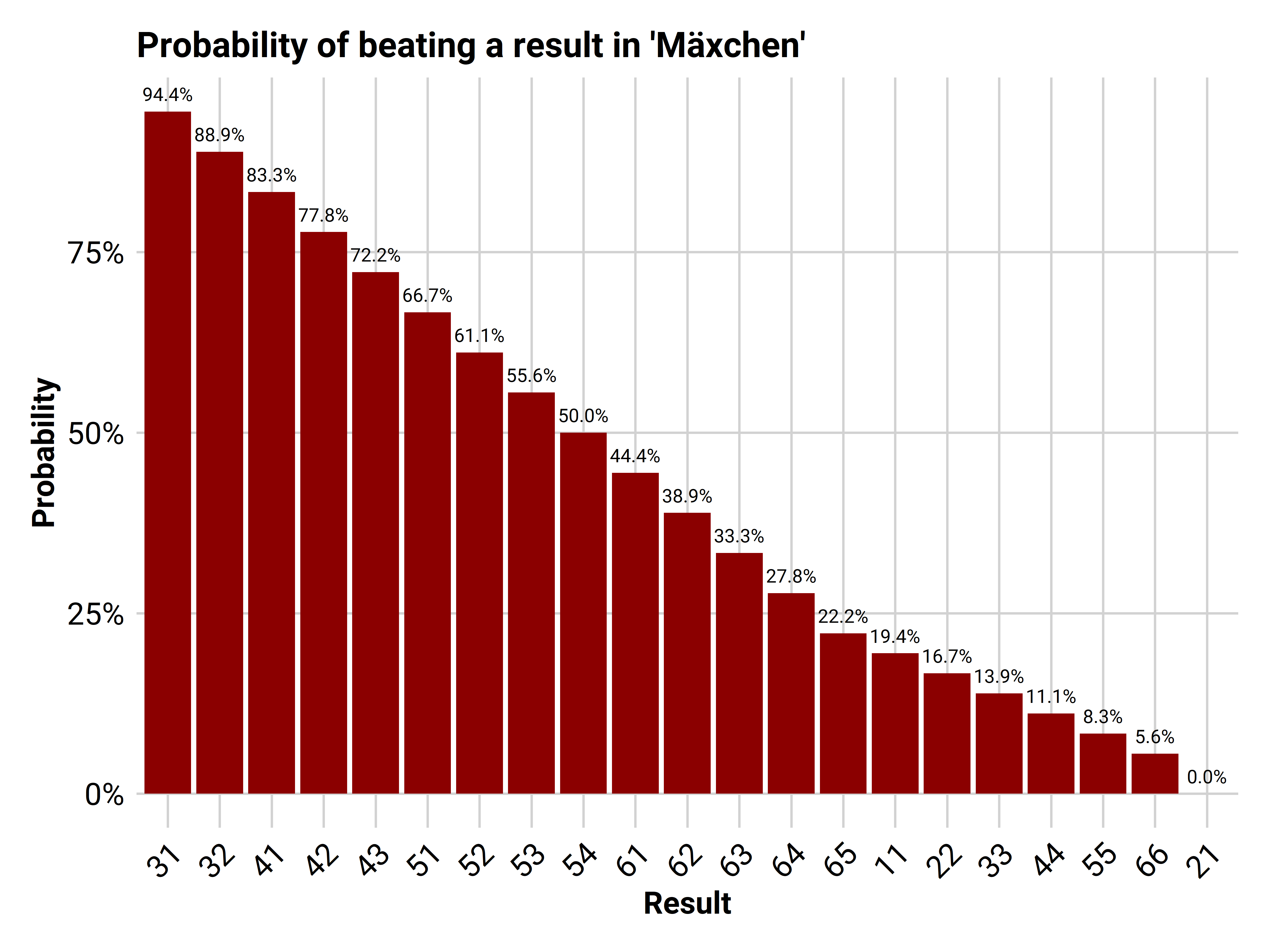

Admittedly, the result is not that surprising and frankly pretty basic math. Though if you wanna know how good your chances of beating a result are, you can look at this pretty plot from now on.