Visualizing the Best Fantasy Football Performances of the 2019 Season
With the Fantasy Football season only a few weeks away, I decided to look back at the 2019 season and the greatest weekly performances.
In this post I will try to visualize the best weekly performances as well as the performance of the best players over the whole season.
Setup
First, we need data. Since I didn’t have fantasy specific data I thought the easiest way to do this is to calculate the fantasy points from the Play-By-Play Data.
You can find this and many more great datasets here.
pbp <- readRDS(url("https://raw.githubusercontent.com/guga31bb/nflfastR-data/master/data/play_by_play_2019.rds"))

pbp <- pbp %>%
  filter(
    season_type == "REG",
    between(week, 1, 16)
  )
pbp
## # A tibble: 43,240 x 333
## play_id game_id old_game_id home_team away_team season_type week posteam
## <dbl> <chr> <chr> <chr> <chr> <chr> <int> <chr>
## 1 1 2019_0~ 2019090804 MIN ATL REG 1 <NA>
## 2 36 2019_0~ 2019090804 MIN ATL REG 1 ATL
## 3 51 2019_0~ 2019090804 MIN ATL REG 1 ATL
## 4 79 2019_0~ 2019090804 MIN ATL REG 1 ATL
## 5 100 2019_0~ 2019090804 MIN ATL REG 1 ATL
## 6 121 2019_0~ 2019090804 MIN ATL REG 1 ATL
## 7 148 2019_0~ 2019090804 MIN ATL REG 1 MIN
## 8 185 2019_0~ 2019090804 MIN ATL REG 1 MIN
## 9 214 2019_0~ 2019090804 MIN ATL REG 1 MIN
## 10 239 2019_0~ 2019090804 MIN ATL REG 1 MIN
## # ... with 43,230 more rows, and 325 more variables: posteam_type <chr>,
## # defteam <chr>, side_of_field <chr>, yardline_100 <dbl>, game_date <chr>,
## # quarter_seconds_remaining <dbl>, half_seconds_remaining <dbl>,
## # game_seconds_remaining <dbl>, game_half <chr>, quarter_end <dbl>,
## # drive <dbl>, sp <dbl>, qtr <dbl>, down <dbl>, goal_to_go <dbl>, time <chr>,
## # yrdln <chr>, ydstogo <dbl>, ydsnet <dbl>, desc <chr>, play_type <chr>,
## # yards_gained <dbl>, shotgun <dbl>, no_huddle <dbl>, qb_dropback <dbl>,
## # qb_kneel <dbl>, qb_spike <dbl>, qb_scramble <dbl>, pass_length <chr>,
## # pass_location <chr>, air_yards <dbl>, yards_after_catch <dbl>,
## # run_location <chr>, run_gap <chr>, field_goal_result <chr>,
## # kick_distance <dbl>, extra_point_result <chr>, two_point_conv_result <chr>,
## # home_timeouts_remaining <dbl>, away_timeouts_remaining <dbl>,
## # timeout <dbl>, timeout_team <chr>, td_team <chr>,
## # posteam_timeouts_remaining <dbl>, defteam_timeouts_remaining <dbl>,
## # total_home_score <dbl>, total_away_score <dbl>, posteam_score <dbl>,
## # defteam_score <dbl>, score_differential <dbl>, posteam_score_post <dbl>,
## # defteam_score_post <dbl>, score_differential_post <dbl>,
## # no_score_prob <dbl>, opp_fg_prob <dbl>, opp_safety_prob <dbl>,
## # opp_td_prob <dbl>, fg_prob <dbl>, safety_prob <dbl>, td_prob <dbl>,
## # extra_point_prob <dbl>, two_point_conversion_prob <dbl>, ep <dbl>,
## # epa <dbl>, total_home_epa <dbl>, total_away_epa <dbl>,
## # total_home_rush_epa <dbl>, total_away_rush_epa <dbl>,
## # total_home_pass_epa <dbl>, total_away_pass_epa <dbl>, air_epa <dbl>,
## # yac_epa <dbl>, comp_air_epa <dbl>, comp_yac_epa <dbl>,
## # total_home_comp_air_epa <dbl>, total_away_comp_air_epa <dbl>,
## # total_home_comp_yac_epa <dbl>, total_away_comp_yac_epa <dbl>,
## # total_home_raw_air_epa <dbl>, total_away_raw_air_epa <dbl>,
## # total_home_raw_yac_epa <dbl>, total_away_raw_yac_epa <dbl>, wp <dbl>,
## # def_wp <dbl>, home_wp <dbl>, away_wp <dbl>, wpa <dbl>, home_wp_post <dbl>,
## # away_wp_post <dbl>, vegas_wp <dbl>, vegas_home_wp <dbl>,
## # total_home_rush_wpa <dbl>, total_away_rush_wpa <dbl>,
## # total_home_pass_wpa <dbl>, total_away_pass_wpa <dbl>, air_wpa <dbl>,
## # yac_wpa <dbl>, comp_air_wpa <dbl>, comp_yac_wpa <dbl>,
## # total_home_comp_air_wpa <dbl>, ...We now have every play of the 2019 NFL season! The dataset is missing fantasy points, so we need to calculate them for the game we are interested in. Since we will reuse this calculation a lot, it’s best to write a function. I will call it calc_ff:
You can use . %>% to create a anonymous function. The function calculates the time, that has progressed since the start of a game in seconds, in order to sort it by this variable. This is necessary because we will use accumulate() to sum up the plays shortly.
After that we will calculate the points. Every yards gained equals a tenth of a point, touchdowns give 6 points, if you fumble you will lose 2 points. This calculation is for the .5PPR format, so each reception will give you half a point. You get 2 points for a successful Two-Point-Conversion.
After that, we accumulate the independent plays in order to get the total fantasy points up to that point.
Lastly, I used the relatively new but awesome function relocate() to display the points in front. We will also create a function to calculate for the whole season.
(Note: This calculation will only work for skill positions, if you would like to analyze Quaterbacks you have to change the function a bit)
calc_ff <- . %>%
  arrange(desc(game_seconds_remaining)) %>%
  mutate(time_in_sec = 3600 - game_seconds_remaining) %>%
  mutate(
    ff_points = yards_gained / 10,
    ff_points = ifelse(touchdown, ff_points + 6, ff_points),
    ff_points = ifelse(fumble_lost, ff_points - 2, ff_points),
    ff_points = ifelse(play_type == "pass" & complete_pass, ff_points + .5, ff_points),
    ff_points = ifelse(two_point_attempt & two_point_conv_result == "success", 2, ff_points),
    ff_points_sum = accumulate(ff_points, sum),
    ff_points_total = last(ff_points_sum)
  ) %>%
  relocate(contains("ff_points"), .before = play_id)

calc_ff_season <- . %>%
  group_by(game_date) %>%
  calc_ff() %>%
  ungroup()
Visualization for NFl related things is a perfect opportunity to try out the package teamcolors.
There is a little bit of setup required to get it to work with our data
library(teamcolors)

# Unfortunately Play-By-Play Data uses Abbreviations while Teamcolors uses full names
team_abbr <- tribble(
  ~name, ~team_code,
  "Arizona Cardinals", "ARI",
  "Atlanta Falcons", "ATL",
  "Baltimore Ravens", "BAL",
  "Buffalo Bills", "BUF",
  "Carolina Panthers", "CAR",
  "Chicago Bears", "CHI",
  "Cincinnati Bengals", "CIN",
  "Cleveland Browns", "CLE",
  "Dallas Cowboys", "DAL",
  "Denver Broncos", "DEN",
  "Detroit Lions", "DET",
  "Green Bay Packers", "GB",
  "Houston Texans", "HOU",
  "Indianapolis Colts", "IND",
  "Jacksonville Jaguars", "JAX",
  "Kansas City Chiefs", "KC",
  "Los Angeles Chargers", "LAC",
  "Los Angeles Rams", "LA",
  "Miami Dolphins", "MIA",
  "Minnesota Vikings", "MIN",
  "New England Patriots", "NE",
  "New Orleans Saints", "NO",
  "New York Giants", "NYG",
  "New York Jets", "NYJ",
  "Oakland Raiders", "LV",
  "Philadelphia Eagles", "PHI",
  "Pittsburgh Steelers", "PIT",
  "San Francisco 49ers", "SF",
  "Seattle Seahawks", "SEA",
  "Tampa Bay Buccaneers", "TB",
  "Tennessee Titans", "TEN",
  "Washington Redskins", "WAS"
)

teamcols <- filter(teamcolors, league == "nfl") %>%
  left_join(team_abbr, by = "name") %>%
  select(team_code, name, primary, secondary, logo)

teamcols
## # A tibble: 32 x 5
## team_code name primary secondary logo
## <chr> <chr> <chr> <chr> <chr>
## 1 ARI Arizona Ca~ #97233f #000000 http://content.sportslogos.net/logos~
## 2 ATL Atlanta Fa~ #a71930 #000000 http://content.sportslogos.net/logos~
## 3 BAL Baltimore ~ #241773 #000000 http://content.sportslogos.net/logos~
## 4 BUF Buffalo Bi~ #00338d #c60c30 http://content.sportslogos.net/logos~
## 5 CAR Carolina P~ #0085ca #000000 http://content.sportslogos.net/logos~
## 6 CHI Chicago Be~ #0b162a #c83803 http://content.sportslogos.net/logos~
## 7 CIN Cincinnati~ #000000 #fb4f14 http://content.sportslogos.net/logos~
## 8 CLE Cleveland ~ #fb4f14 #22150c http://content.sportslogos.net/logos~
## 9 DAL Dallas Cow~ #002244 #b0b7bc http://content.sportslogos.net/logos~
## 10 DEN Denver Bro~ #002244 #fb4f14 http://content.sportslogos.net/logos~
## # ... with 22 more rowsNow that we have the team abbreviations we can join with our dataset:
pbp <- pbp %>% left_join(teamcols, by = c("posteam" = "team_code"))We are finally ready to do some visualization.
Visualization of weekly perfomances
As discussed earlier in this post, we will reuse the same plot a few times, so we should just write a function for it. We want to plot the performance of a player for a given week so those will be our arguments along with a plot title.
I also would like to make the graph interactive, using the plotly package.
First we filter out only the plays for our player (using his id) and the given week. The dataset now only contains plays from the specified week, where the player was involved as a receiver or runner, so on this data we can run our function to calculate his fantasy points.
text_disp will contain the text, that we want to display if you hover over an event. Events are either a Touchdown, which we will display as a red dot or a fumble, which will be a black dot.
The Line, that shows the Fantasy Points over Game Time will be colored in the primary color of the players team.
Each quater will be seperated by a dashed vline. The rest of the code is necessary so that plotly won’t display labels for the time axis.
Edit: Unfortunately Plotly does not seem to work in this environment, Plotly Plot will display, but in completely wrong dimensions. Therefore I will comment out the Plotly Part. The Rest won’t be changed so you could just run ggplotly(p, tooltip = "text") on your plot.
# library(plotly)

plot_week_performance <- function(player_id, week_nr, plot_title) {
  p <- pbp %>%
    filter(
      receiver_player_id == player_id | rusher_player_id == player_id,
      week == week_nr
    ) %>%
    calc_ff() %>%
    arrange(time_in_sec) %>%
    mutate(text_disp = glue::glue("Quater: {qtr}\nDrive: {drive}\nTime: {time}\n\nScore\n{away_team}: {total_away_score}\n{home_team}: {total_home_score}\n")) %>%
    ggplot(aes(time_in_sec, ff_points_sum, color = primary)) +
    geom_line(size = 1) +
    geom_point(
      shape = 19, color = "red", size = 2, data = . %>% filter(touchdown == T),
      aes(time_in_sec, ff_points_sum, text = text_disp)
    ) +
    geom_point(
      shape = 19, color = "black", size = 2, data = . %>% filter(fumble == T),
      aes(time_in_sec, ff_points_sum, text = text_disp)
    ) +
    geom_vline(xintercept = c(900, 1800, 2700), alpha = .5, lty = 2) +
    expand_limits(x = c(0, 3600)) +
    scale_x_continuous(labels = NULL, breaks = NULL) +
    scale_color_identity() +
    theme_hubnr_thin() +
    labs(
      title = plot_title,
      x = "Time",
      y = "Fantasy Points"
    ) +
    theme(
      legend.position = "none",
      axis.ticks.x = element_blank(),
      axis.text.x = element_blank()
    )

  # ggplotly(p, tooltip = "text")
  p
}
Now that we have our plot generating function, we should test it on some of the best fantasy performances of the last season.
In order to get results you need a player_id, which you can get by filtering the dataset for the specific player (Hint: Kenyan Drake would be ‘K.Drake’). I will omit this step for this post.
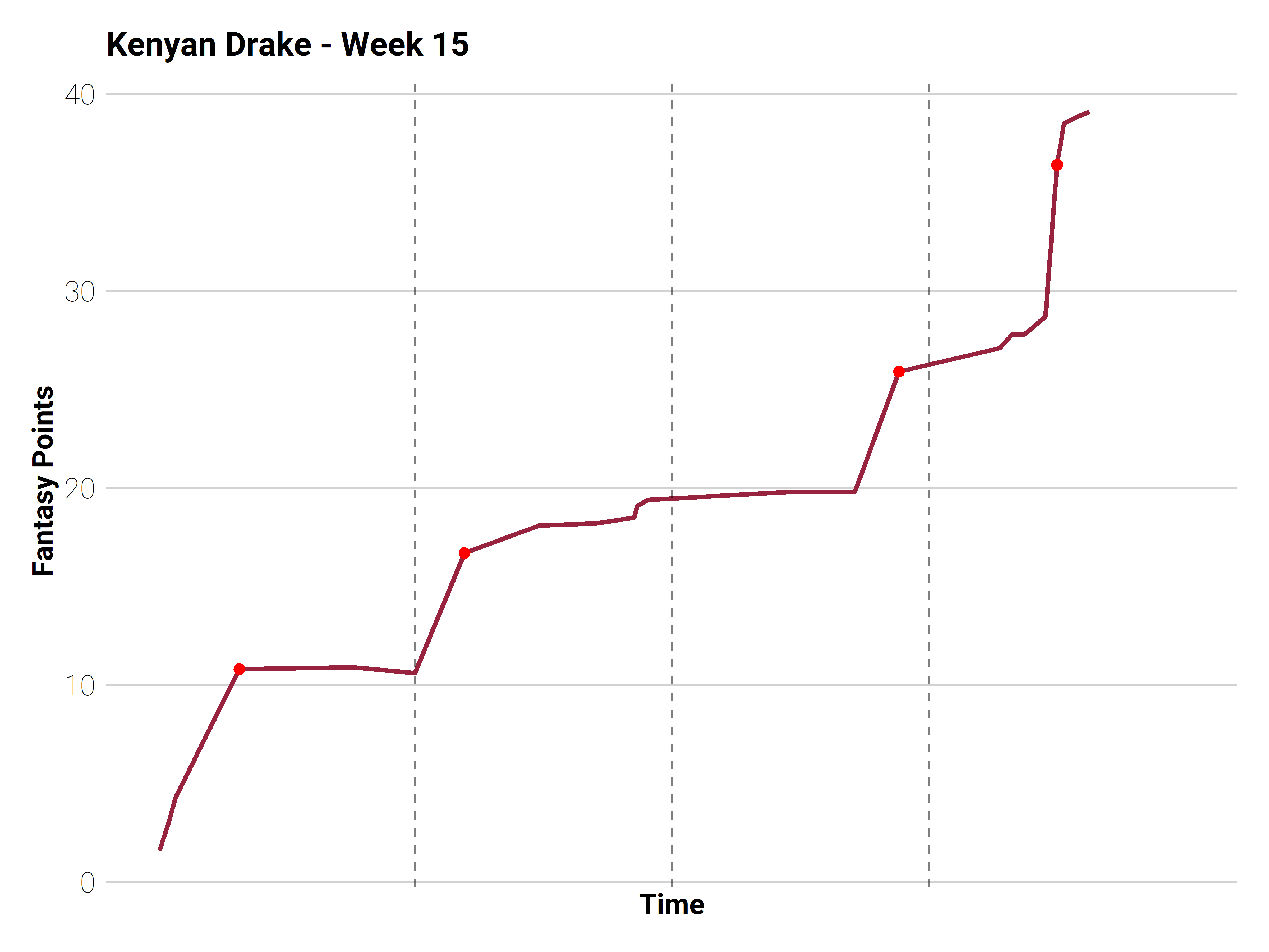
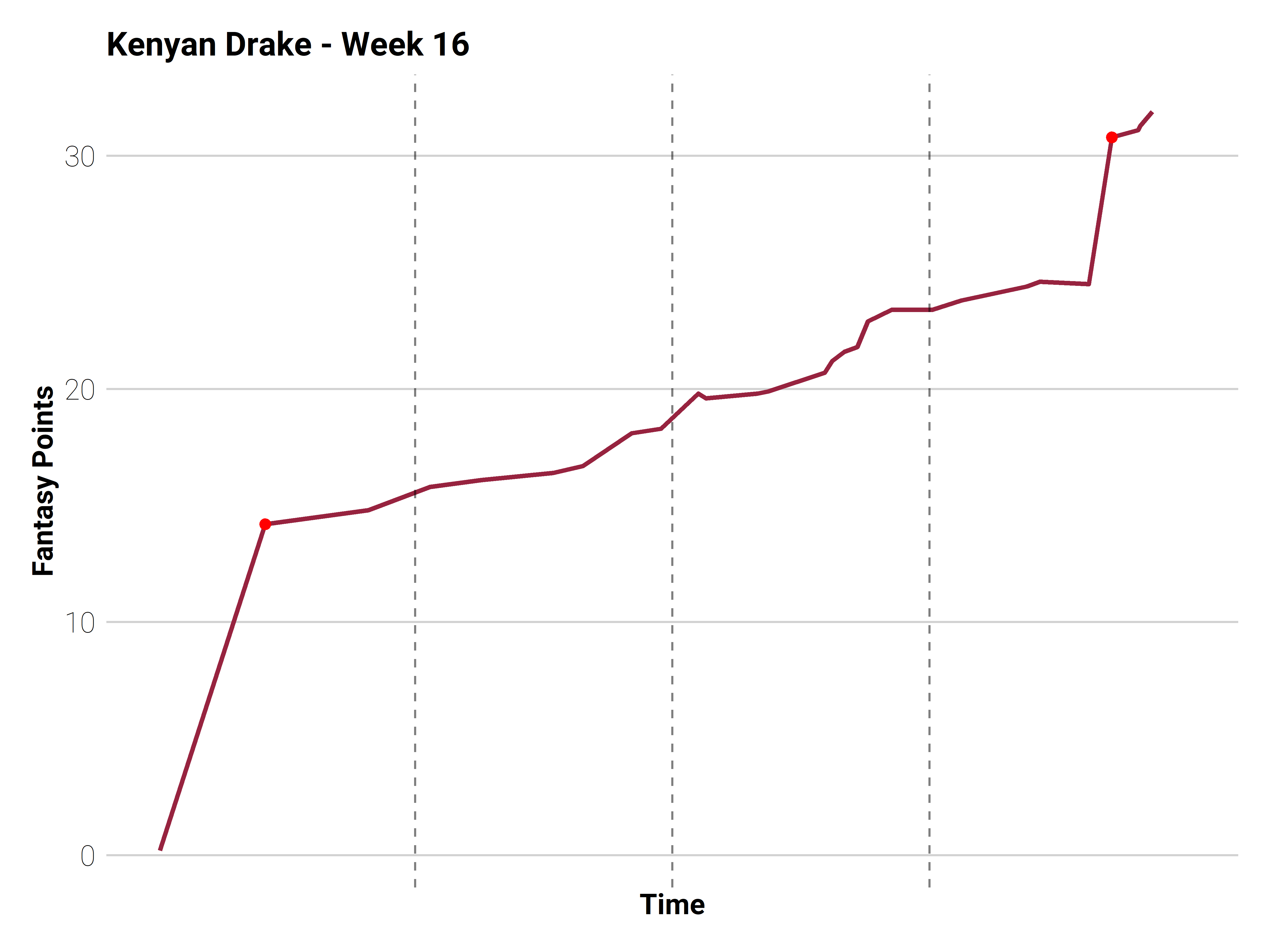
Kenyan Drake - Week 15 (and 16)
Let’s start with Kenyan Drake. After a disappointing first half of the season on the Miami Dolphins, Drake got traded to the Arizona Cardinals, where he became fantasy gold immediatly. Especially his performances in the Fantasy Football playoffs made Kenyan Drake a League Winner
plot_week_performance(
  "32013030-2d30-3033-3331-31385a388006", 15,
  "Kenyan Drake - Week 15"
)
plot_week_performance(
  "32013030-2d30-3033-3331-31385a388006", 16,
  "Kenyan Drake - Week 16"
)
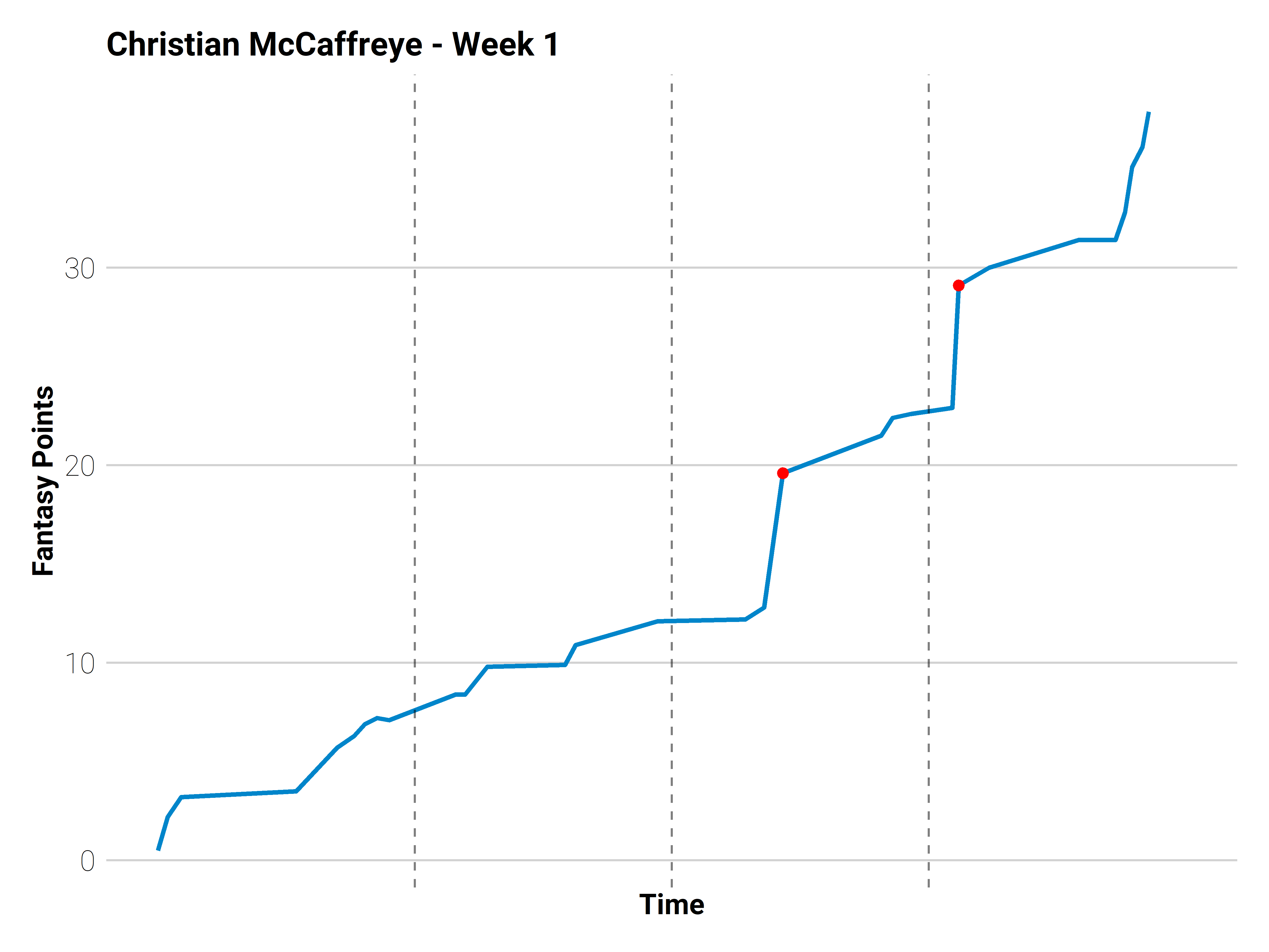
Christian McCaffrey - Week 1
McCaffrey was awesome the whole season long (execpt week 2). He started the season off with an incredible performance, racking up 42.9 fantasy points. The insane thing about McCaffreys season is, that this wasn’t even his best fantasy performance (47.7 pts - Week 5 vs. Jax).
plot_week_performance(
  "32013030-2d30-3033-3332-3830ec2c3be7", 1,
  "Christian McCaffreye - Week 1"
)
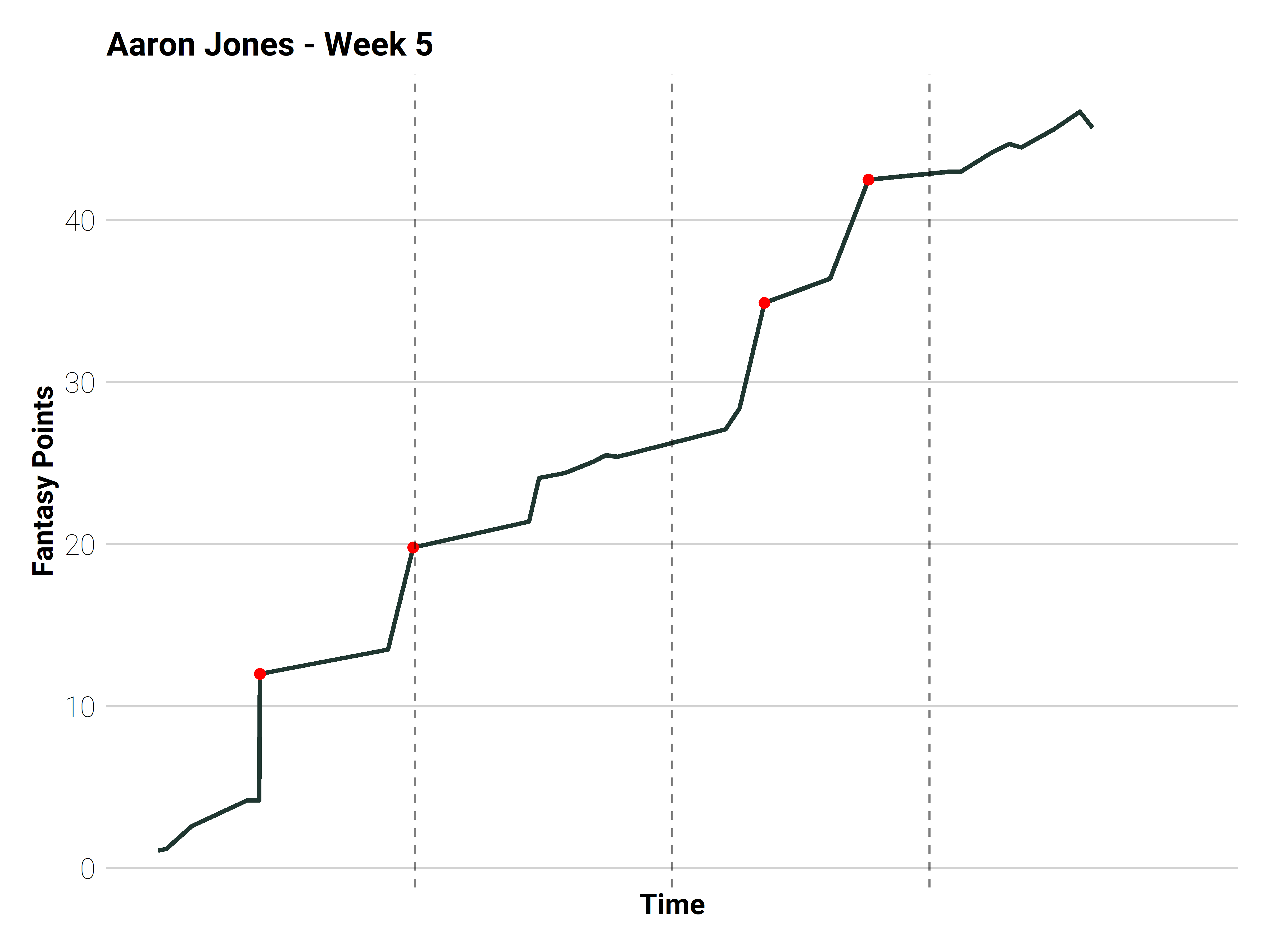
Aaron Jones - Week 5
Aaron Jones performance in Week 5 was spectacular. He was the running back, that scored the most points in a single game this season.
plot_week_performance(
  "32013030-2d30-3033-3332-3933ed82c0de", 5,
  "Aaron Jones - Week 5"
)
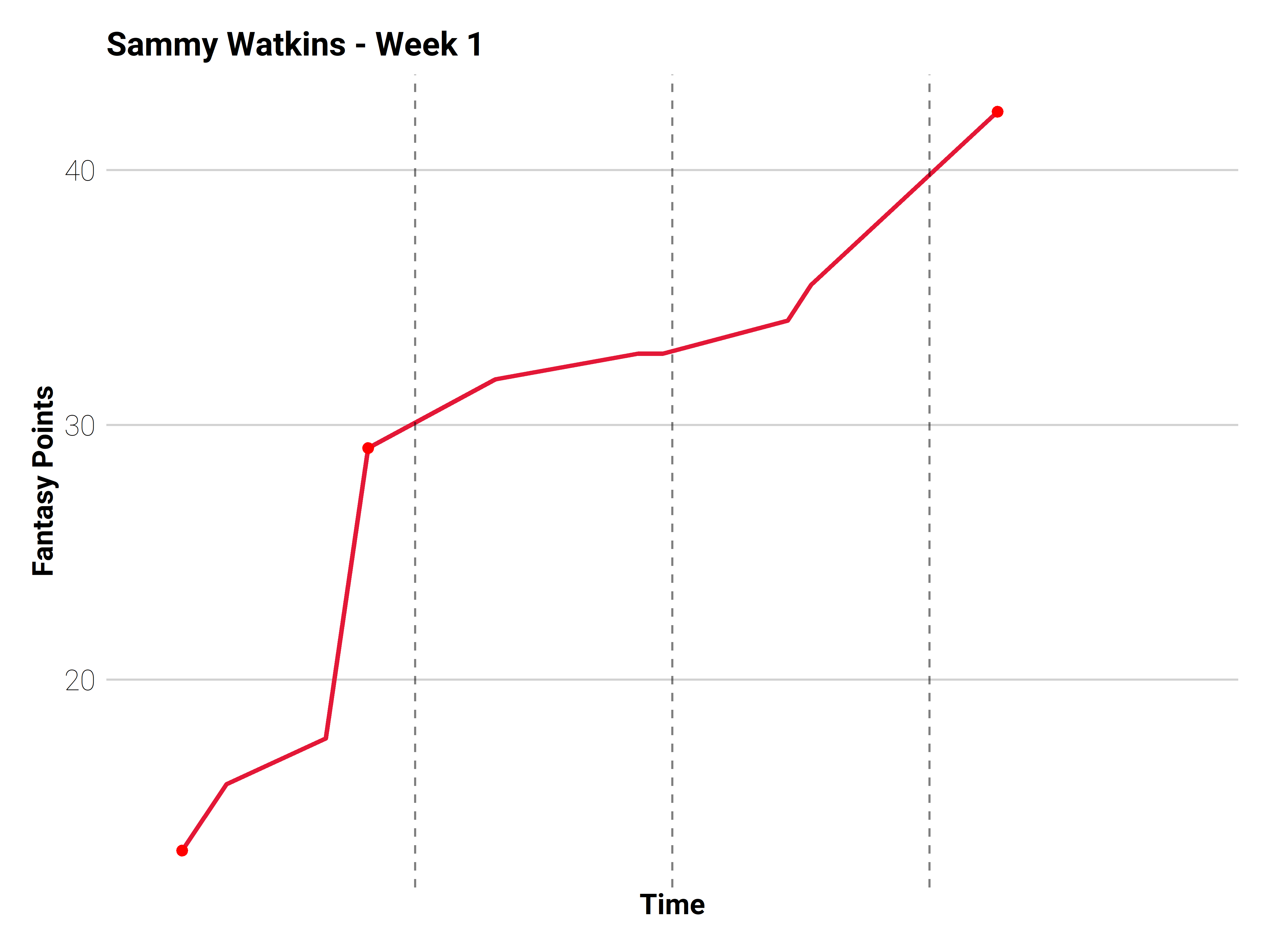
Sammy Watkins - Week 1
Similar to McCaffrey, Sammy Watkins hat an unbelivable first week, scoring 46.8 points! Unfortuantely, unlike McCaffrey, he could not reproduce a similar performance again. In fact, Watkins Week 1 performance contributed more than a quater of his total points this season.
plot_week_performance(
  "32013030-2d30-3033-3133-32353107e672", 1,
  "Sammy Watkins - Week 1"
)
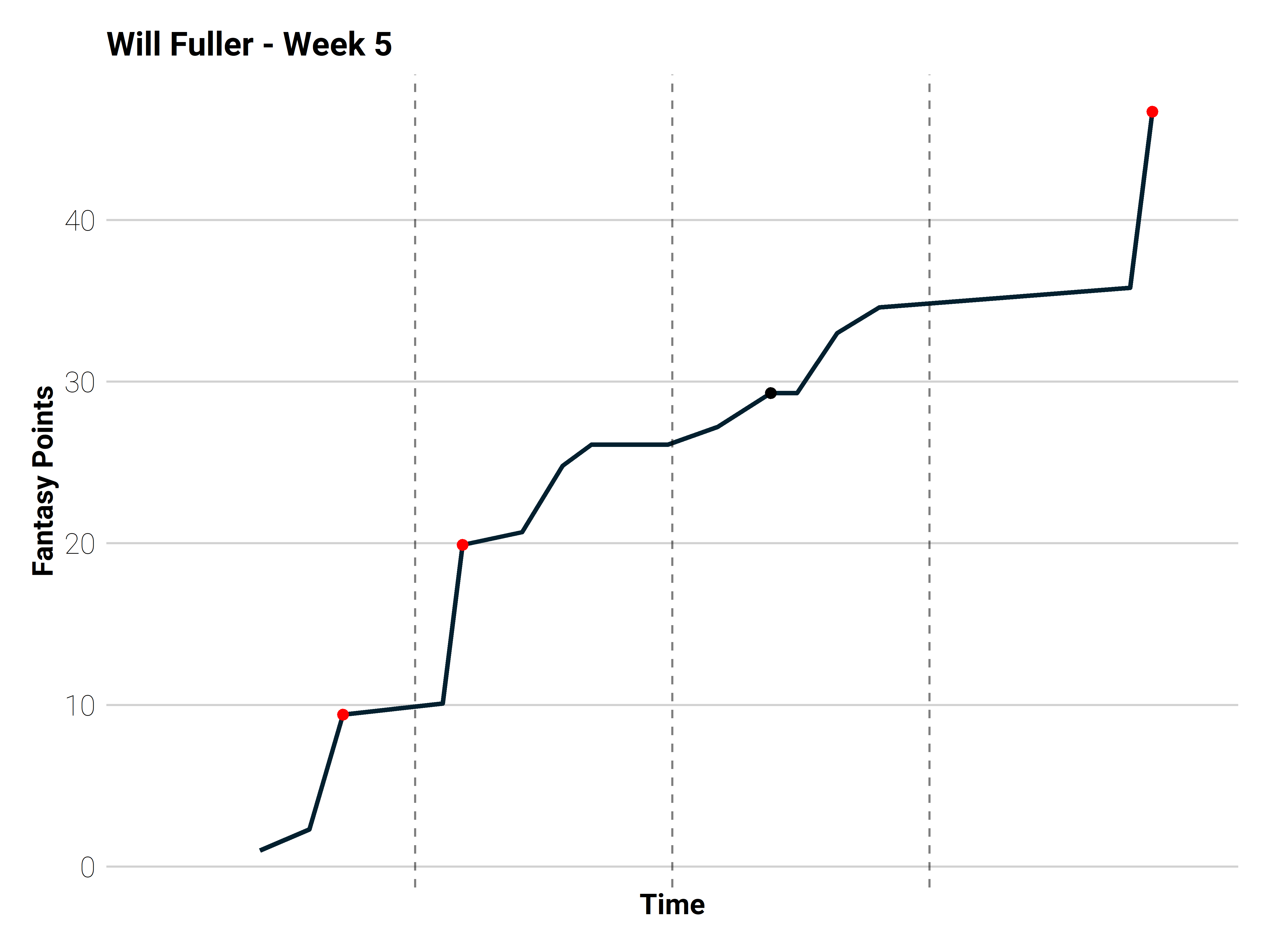
Will Fuller - Week 5
Similar to Watkins, Fuller also had one week, that outshined the rest of his season by a mile. He scored the most fantasy points in a game for a Wide Receiver this Year (53.7)
plot_week_performance(
  "32013030-2d30-3033-3331-3237332aee05", 5,
  "Will Fuller - Week 5"
)
Visualization of season perfomance
Now that we looked at individual games, let’s have a look at the whole season of a player.
To do that we need to create one of these plots for every game and display them together using facet_wrap().
Let’s create a function again. It’s will be very similar to the game plot function only a few things are different. We will color the odd weeks in the primary color and the even weeks in the secondary color of the players NFL team. We also need to convert week to factor in order to sort the facets.
plot_season_performance <- function(player_id, plot_title) {
  pbp %>%
    filter(receiver_player_id == player_id | rusher_player_id == player_id) %>%
    calc_ff_season() %>%
    arrange(week) %>%
    mutate(
      line_color = ifelse(week %% 2 == 1, primary, secondary),
      week_nr = week,
      week = glue::glue("Week {week} ({ff_points_total})")
    ) %>%
    mutate_at(vars(week), funs(factor(., levels = unique(.)))) %>%
    ggplot(aes(time_in_sec, ff_points_sum)) +
    geom_line(aes(color = line_color), size = 1) +
    geom_point(
      shape = 19, color = "red", size = 2, data = . %>% filter(touchdown == T),
      aes(time_in_sec, ff_points_sum)
    ) +
    geom_point(
      shape = 19, color = "red", size = 2, data = . %>% filter(touchdown == T),
      aes(time_in_sec, ff_points_sum)
    ) +
    scale_color_identity() +
    facet_wrap(~week) +
    geom_vline(xintercept = c(900, 1800, 2700), alpha = .5, lty = 2) +
    expand_limits(x = c(0, 3600)) +
    scale_x_continuous(labels = NULL, breaks = NULL) +
    theme_hubnr_thin(11) +
    labs(
      title = plot_title,
      x = NULL,
      y = "Fantasy Points"
    ) +
    theme(strip.text.x = element_text(size = 11, face = "plain"))
}
Now we are able to look at performances over a whole season.
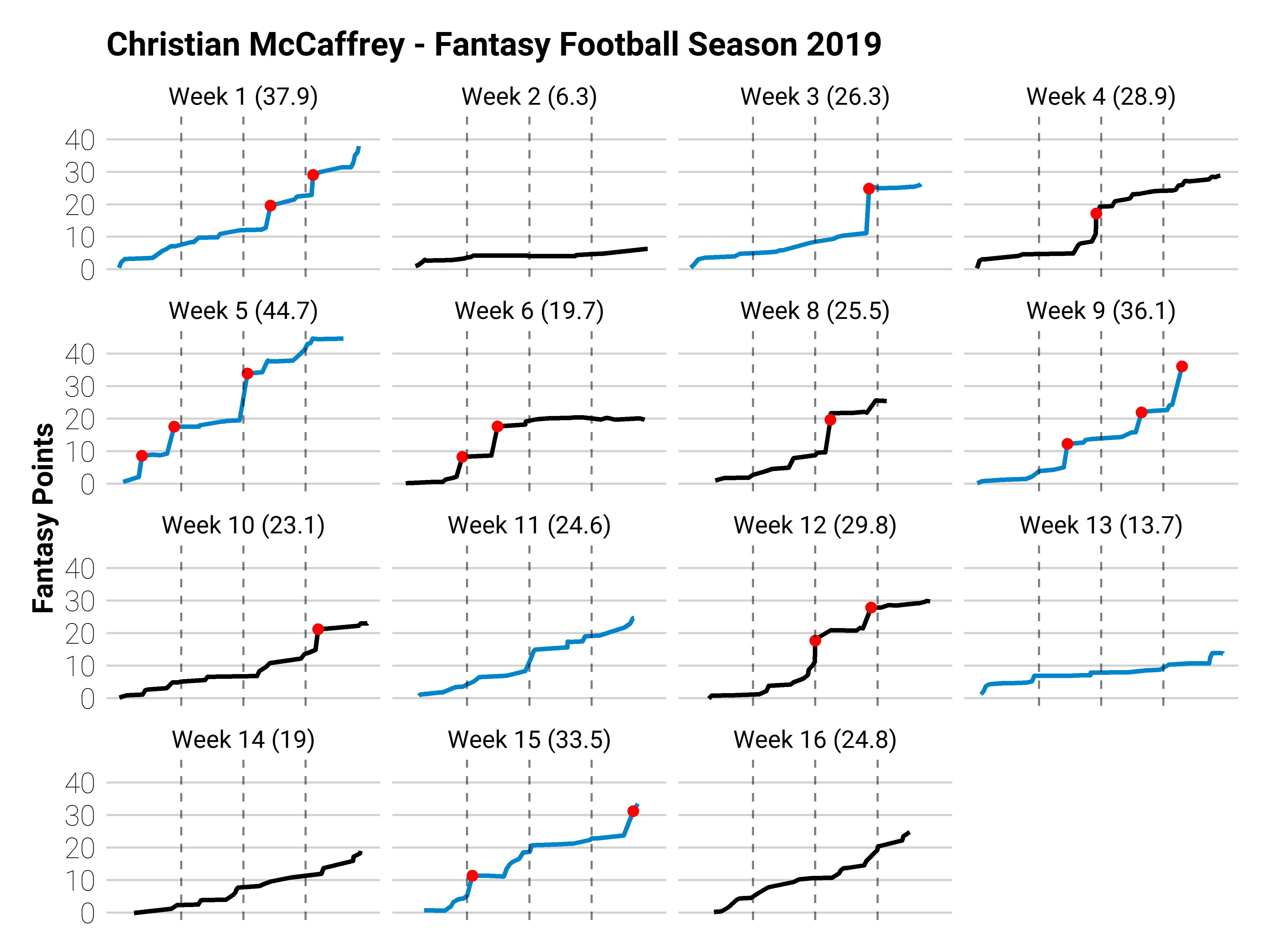
Christian McCaffrey
Without a doubt the most valuable Running Back this season was Christian McCaffrey. Execpt for the previously mentioned Week 2 (and maybe Week 13) he was always great.
plot_season_performance(
  "32013030-2d30-3033-3332-3830ec2c3be7",
  "Christian McCaffrey - Fantasy Football Season 2019"
)
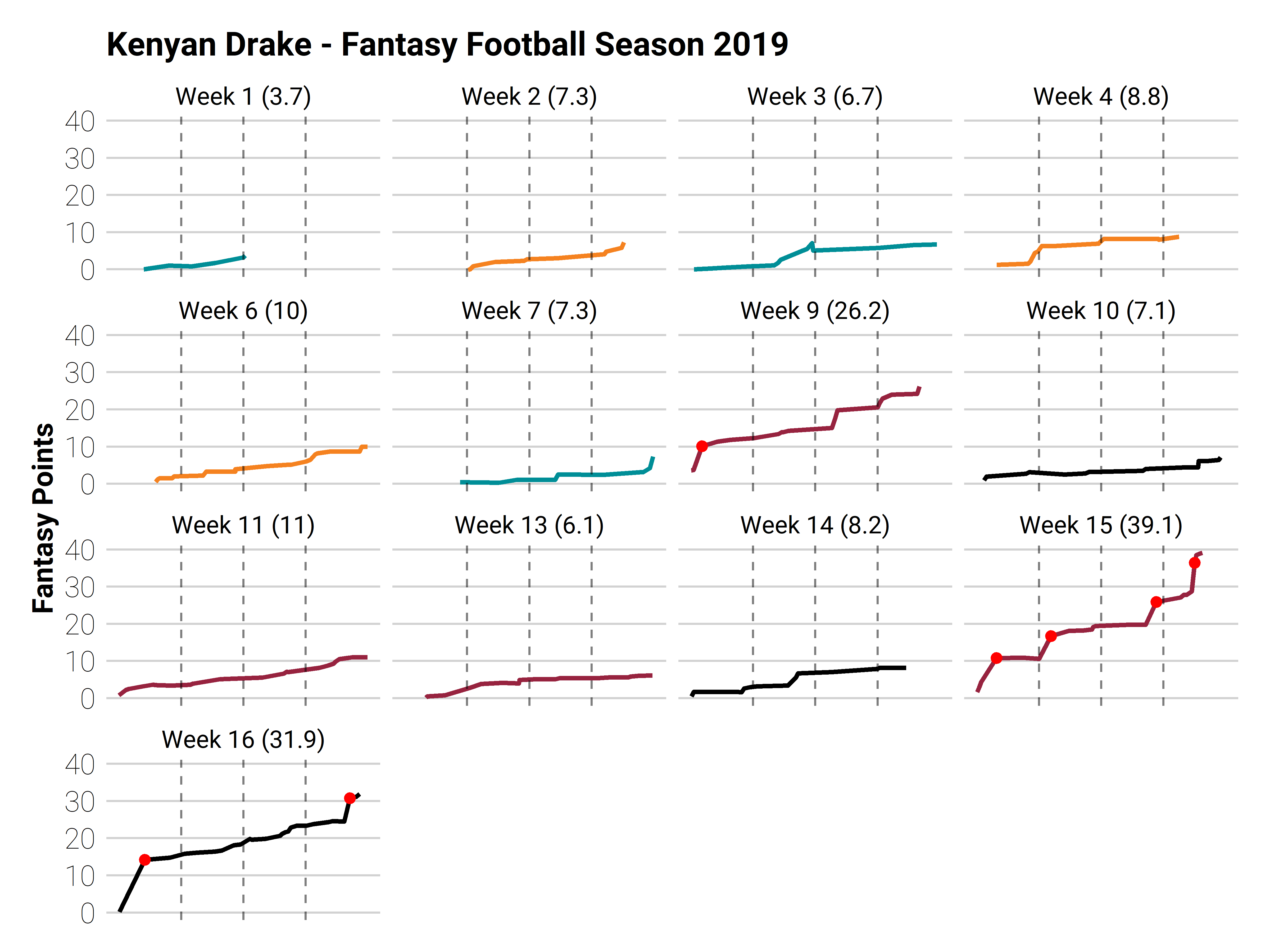
Kenyan Drake
As mentioned earlier Drake had a bad first half, so his season wasn’t that great. I mainly picked him because you can see how the coloring work. Drake was on the Dolphins for the first 8 weeks of the season and after that played for the Cardinals. You can see the coloring of the plot chaning accordingly.
plot_season_performance(
  "32013030-2d30-3033-3331-31385a388006",
  "Kenyan Drake - Fantasy Football Season 2019"
)
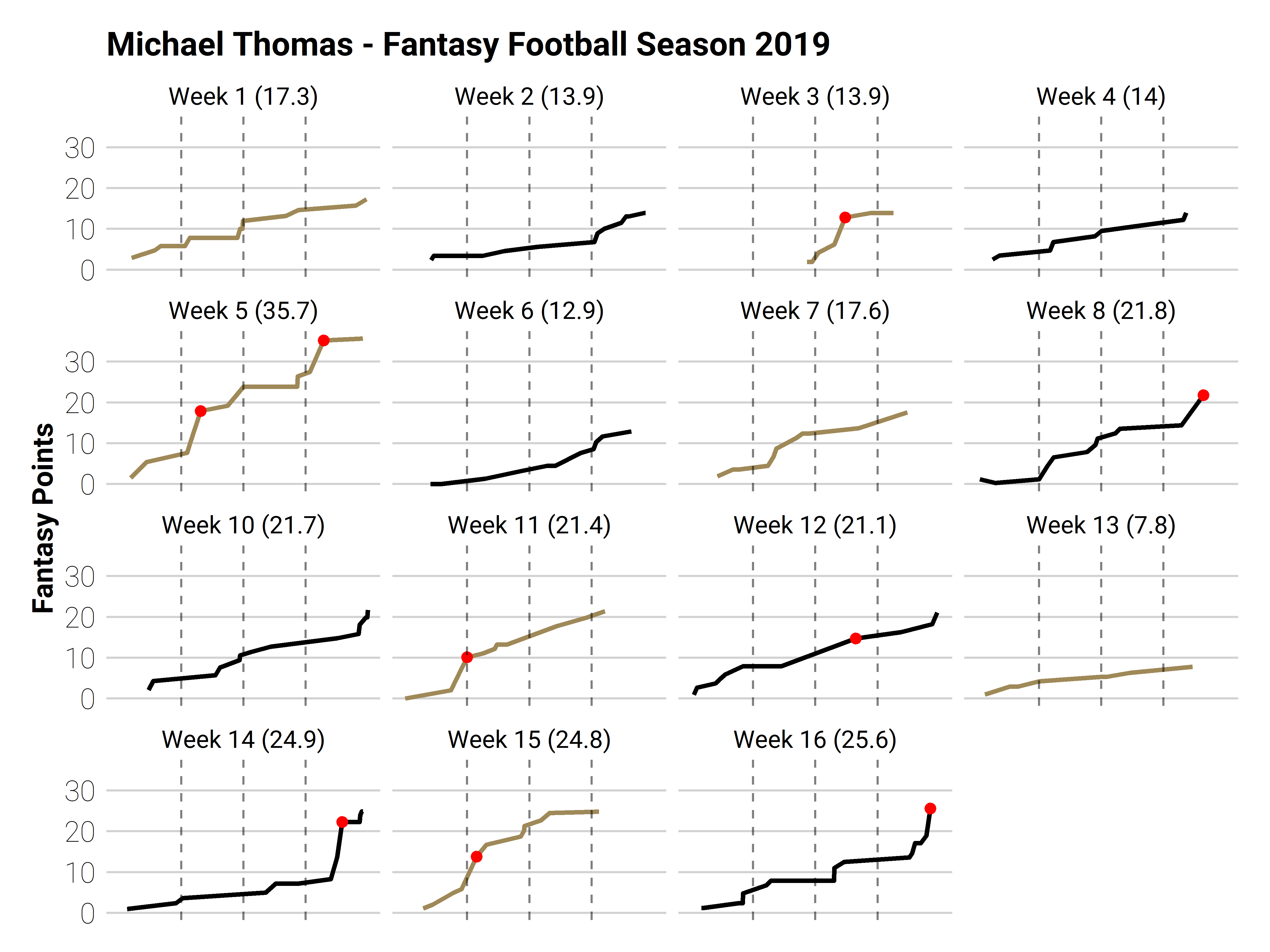
Michael Thomas
Michael Thomas was the best Wide Receiver for Fantasy in the 2019 season.
plot_season_performance(
  "32013030-2d30-3033-3237-36359afa5261",
  "Michael Thomas - Fantasy Football Season 2019"
)
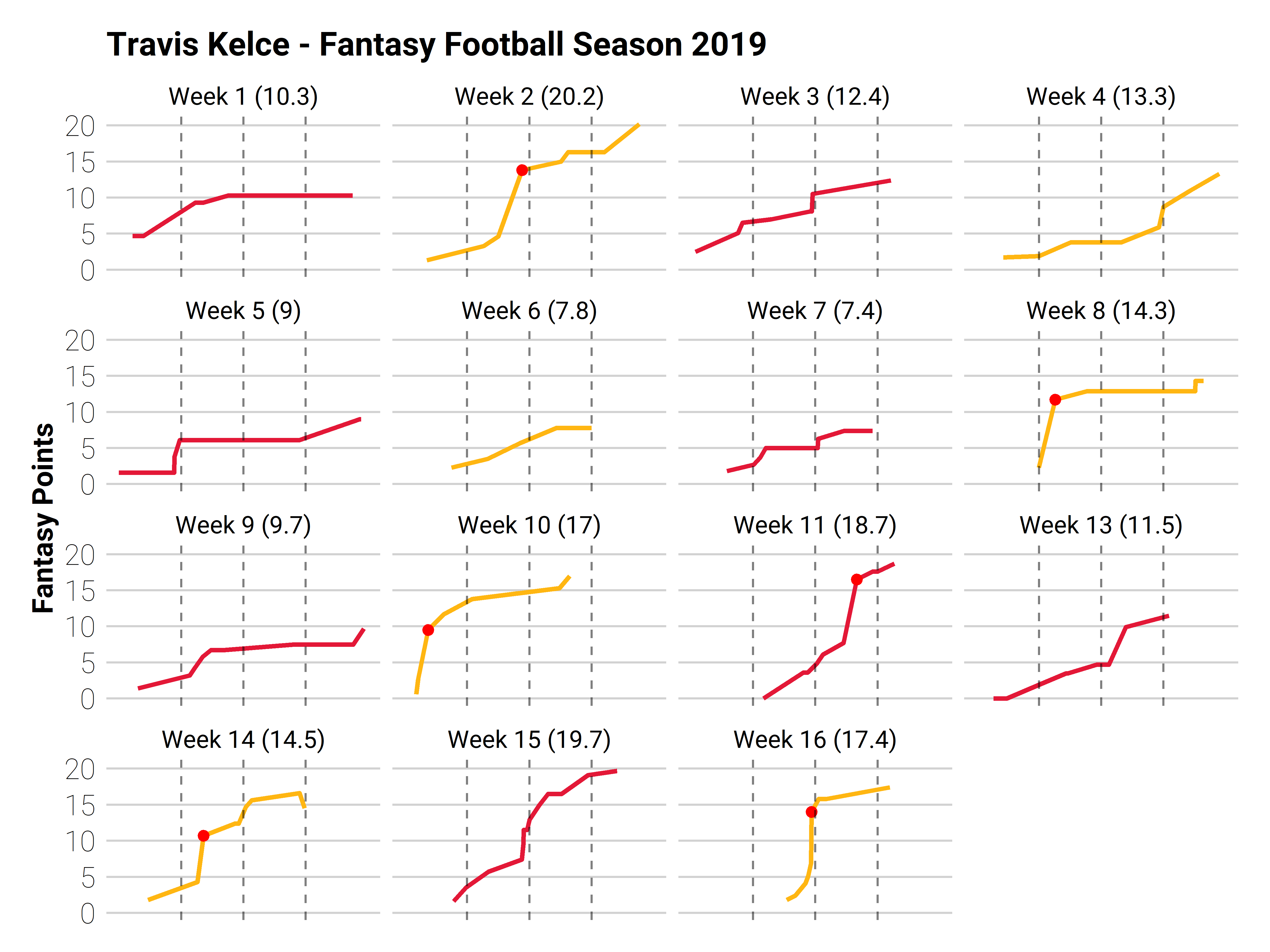
Travis Kelce
Travis Kelce was the best Tight End for Fantasy in the 2019 season.
plot_season_performance(
  "32013030-2d30-3033-3035-3036654ef292",
  "Travis Kelce - Fantasy Football Season 2019"
)